Primvars

A primvar is a special type of attribute that can interpolate the value of the attribute over the surface/volume of a geometric prim. Primvars are most commonly used to communicate per-primitive overrides to shaders/materials for rendering (e.g. providing texture coordinates for a surface), but can be used wherever a surface or volume-varying signal is needed.

Primvar Interpolation Modes

USD currently supports five primvar interpolation modes:

• constant

• uniform

• varying

• vertex

• faceVarying

Each interpolation mode is described in more detail below. Example scenes are provided that use a Mesh Gprim that consists of two quads, along with a primvar for displayColor, to help visualize the interpolation modes via Hydra/Storm (screenshots are from usdview).

Constant Interpolation

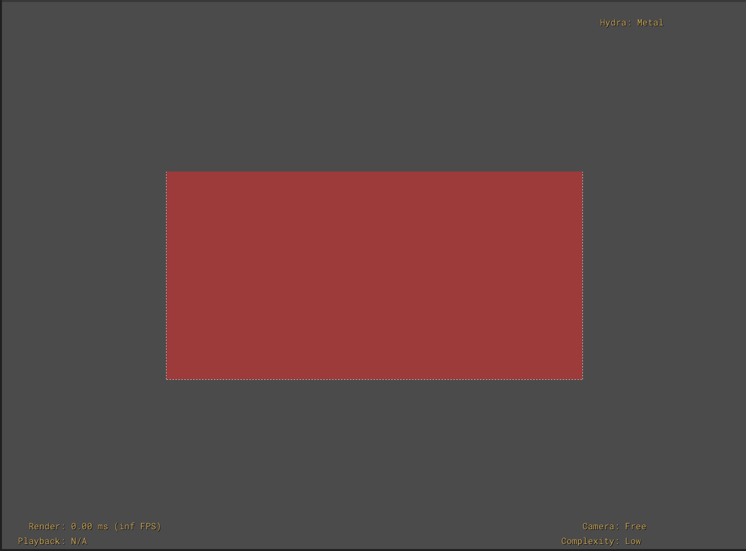
A single element is specified across the entire prim surface/volume. Note that you still need to provide an array (that contains a single element) for the primvar.

In our example we author the displayColor primvar using an array with a single color, and Hydra/Storm renders all the mesh faces with the single color.

#usda 1.0
(
)

def Mesh "constant"
{
   float3[] extent = [(-1, 0, 0), (1, 1, 0)]
   point3f[] points = [(-1, 0, 0), (-1, 1, 0), (0, 1, 0), (0, 0, 0), (1, 1, 0), (1, 0, 0)]
   int[] faceVertexCounts = [4, 4]
   int[] faceVertexIndices = [3, 2, 1, 0, 5, 4, 2, 3]

   color3f[] primvars:displayColor = [(1, 0, 0)] (
       interpolation = "constant"
   )

   double3 xformOp:translate = (0, 0, -10)
   uniform token[] xformOpOrder = ["xformOp:translate"]
}

Uniform Interpolation

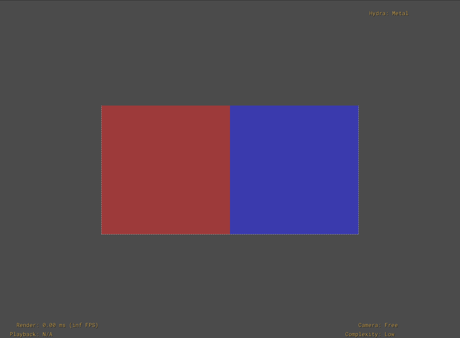
One element remains constant for each patch segment of the prim’s surface/volume. For a mesh prim, provide an array with a single element for each face of the mesh. For a curve prim, provide an array with a single element for each curve segment (as described in UsdGeomBasisCurves – Primvar Interpolation).

The elements in the array must match the count and order of the segments of the prim. For a Mesh prim, the primvar array must have the same number and order of elements as the Mesh’s faceVertexCounts array.

In our example mesh with two faces (quads), we author an array with two colors for the displayColor primvar, and the primvar specifies the appropriate color for each face.

#usda 1.0
(
)

def Mesh "uniform"
{
    float3[] extent = [(-1, 0, 0), (1, 1, 0)]
    point3f[] points = [(-1, 0, 0), (-1, 1, 0), (0, 1, 0), (0, 0, 0), (1, 1, 0), (1, 0, 0)]
    int[] faceVertexCounts = [4, 4]
    int[] faceVertexIndices = [3, 2, 1, 0, 5, 4, 2, 3]

    color3f[] primvars:displayColor = [(1, 0, 0), (0,0,1)] (
        interpolation = "uniform"
    )

    double3 xformOp:translate = (0, 0, -10)
    uniform token[] xformOpOrder = ["xformOp:translate"]
}

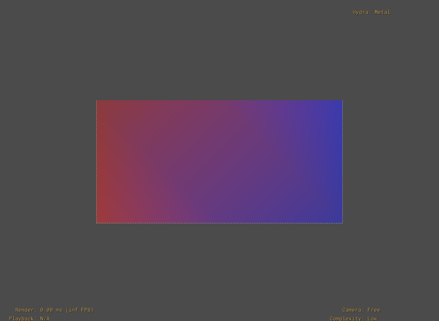
Vertex Interpolation

Elements are interpolated by applying the surface or curve basis functions.

For Mesh prims, you’ll provide a primvar array with one element for each point of the mesh, with the order of the primvar array matching the order of the Mesh points array.

Note

Meshes are defined in terms of points that are connected into edges and faces. Many references to meshes use the term ‘vertex’ in place of or interchangeably with ‘points’, while some use ‘vertex’ to refer to the ‘face-vertices’ that define a face. To avoid confusion, the term ‘vertex’ is intentionally avoided in favor of ‘point’ or ‘face vertex’.

For BasisCurves, you’ll provide a primvar array with one element for each point of the curve, matching the order of the prim’s points array.

In our example Mesh with two faces, we author an array with six colors (matching the Mesh points array count and order). Hydra/Storm renders the Mesh with vertex interpolation going from red at (-1,0,0) to blue at (1,1,0).

#usda 1.0
(
)

def Mesh "vertex"
{
    float3[] extent = [(-1, 0, 0), (1, 1, 0)]
    point3f[] points = [(-1, 0, 0), (-1, 1, 0), (0, 1, 0), (0, 0, 0), (1, 1, 0), (1, 0, 0)]
    int[] faceVertexCounts = [4, 4]
    int[] faceVertexIndices = [3, 2, 1, 0, 5, 4, 2, 3]

    color3f[] primvars:displayColor = [(1, 0, 0), (0.75,0,0), (0.5,0,0.25), (0.25,0,0.5), (0,0,1), (0,0,0.75)] (
        interpolation = "vertex"
    )

    double3 xformOp:translate = (0, 0, -10)
    uniform token[] xformOpOrder = ["xformOp:translate"]
}

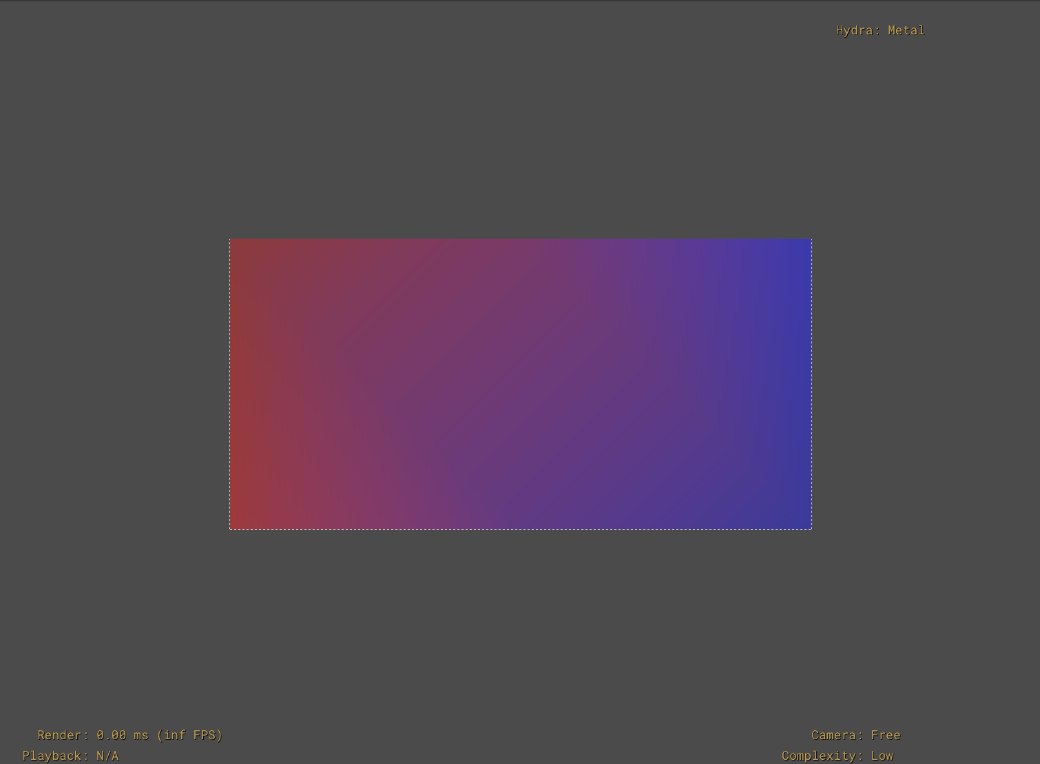
Varying Interpolation

Elements are interpolated over each surface patch or curve segment using linear basis functions. Bilinear or barycentric interpolation is used to interpolate over quad surface patches or triangulated mesh faces respectively. Linear interpolation is used to interpolate over curve segments.

For Mesh prims, you’ll provide a primvar array with one element for each point of the mesh, with the order of the primvar array matching the order of the Mesh points array. Using varying interpolation to set color elements for mesh points is similar to setting “vertex colors” in game engines.

For BasisCurves, you’ll provide a primvar array with two elements for each curve segment. The number of segments will depend on the curve type, wrap (periodicity), and curveVertexCounts values of your curve, as described in the tables in UsdGeomBasisCurves – Primvar Interpolation.

In our example Mesh with two faces, we author an array with six colors (matching the Mesh points array count and order). Hydra/Storm renders the Mesh with varying interpolation going from red at (-1,0,0) to blue at (1,1,0).

#usda 1.0
(
)

def Mesh "varying"
{
    float3[] extent = [(-1, 0, 0), (1, 1, 0)]
    point3f[] points = [(-1, 0, 0), (-1, 1, 0), (0, 1, 0), (0, 0, 0), (1, 1, 0), (1, 0, 0)]
    int[] faceVertexCounts = [4, 4]
    int[] faceVertexIndices = [3, 2, 1, 0, 5, 4, 2, 3]

    color3f[] primvars:displayColor = [(1, 0, 0), (0.75,0,0), (0.5,0,0.25), (0.25,0,0.5), (0,0,1), (0,0,0.75)] (
        interpolation = "varying"
    )

    double3 xformOp:translate = (0, 0, -10)
    uniform token[] xformOpOrder = ["xformOp:translate"]
}

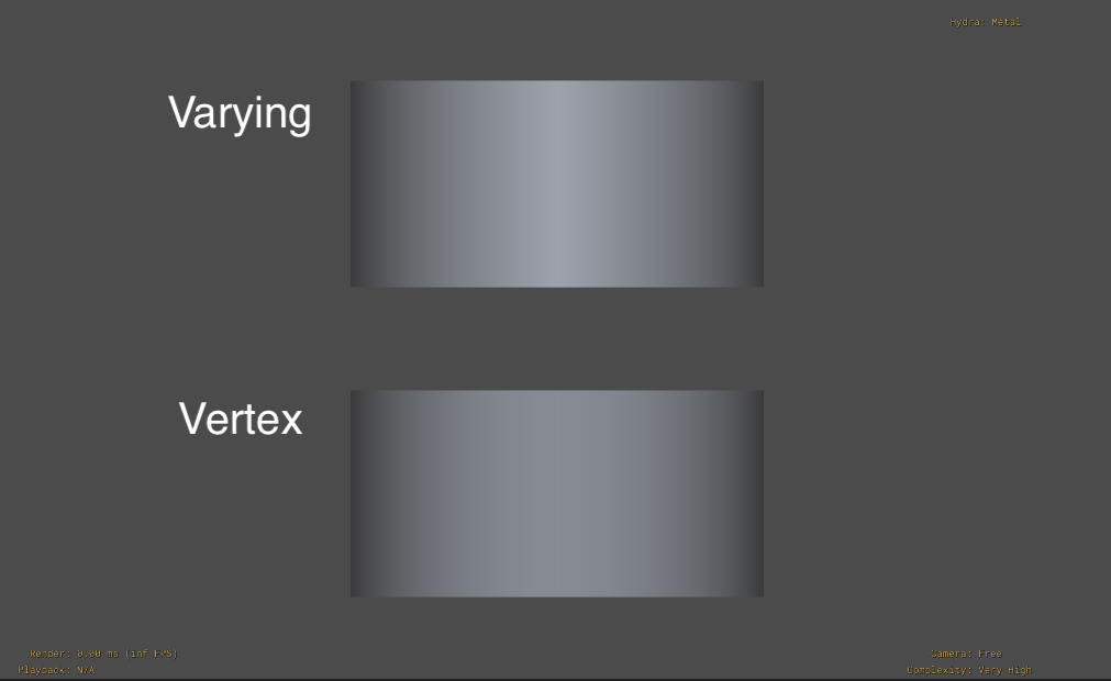
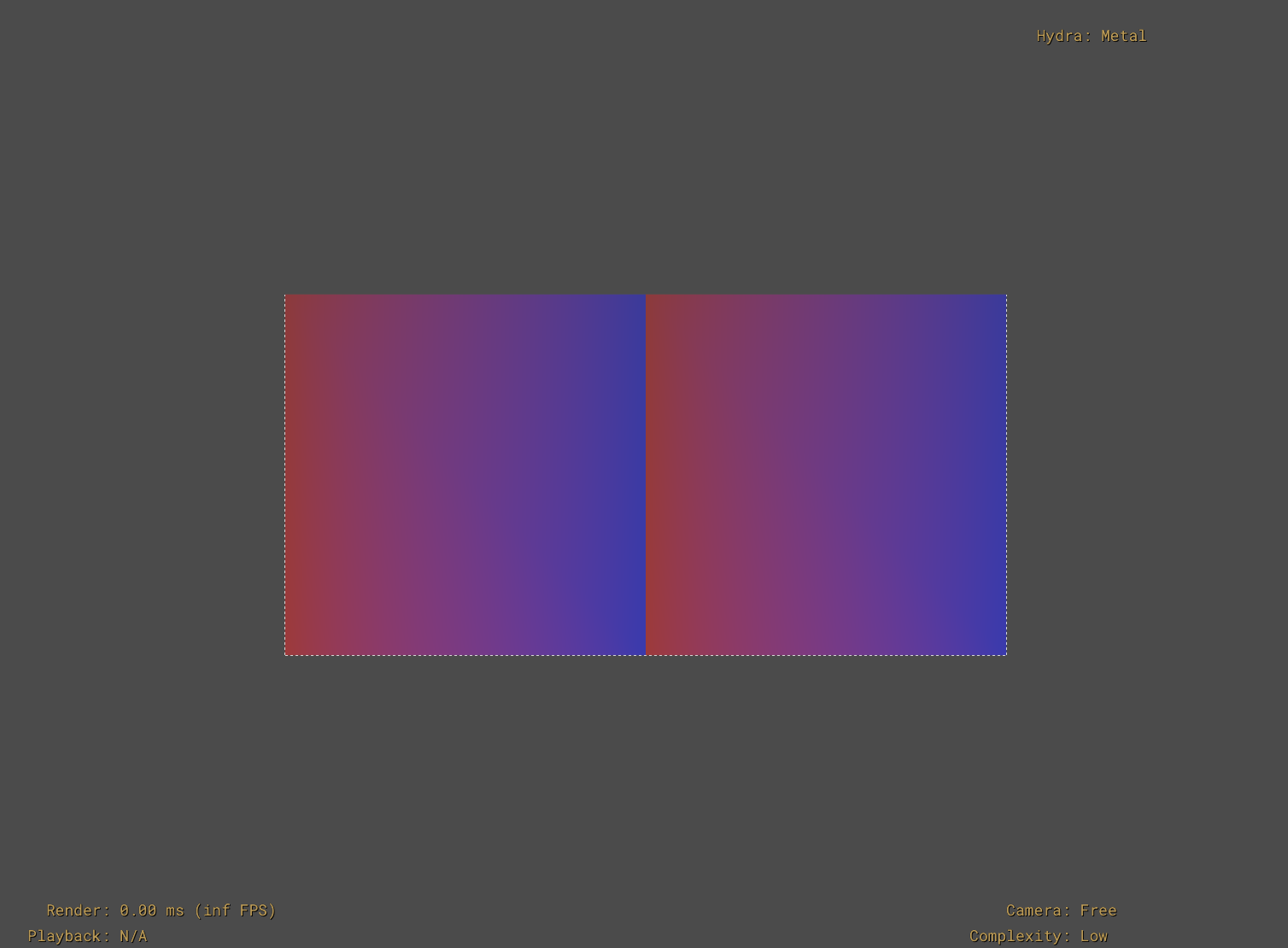
Notice that the example output looks similar to the vertex interpolation Mesh example. The difference between varying and vertex interpolation can be subtle. As vertex interpolation uses the basis function of the prim’s surface or curve, we can visualize the difference if we adjust how our Mesh prim is subdivided. The following example shows the same two-quad Mesh prim using varying and vertex interpolation, with displayColor primvars going from black to white. Rendering this using usdview with --complexity veryhigh shows how the vertex interpolation across a highly subdivided surface follows a smoother gradient, whereas the varying interpolation results in a more linear gradient.

#usda 1.0
(
)

def Mesh "varying"
{
    float3[] extent = [(-1, 0, 0), (1, 1, 0)]
    point3f[] points = [(-1, 0, 0), (-1, 1, 0), (0, 1, 0), (0, 0, 0), (1, 1, 0), (1, 0, 0)]
    int[] faceVertexCounts = [4, 4]
    int[] faceVertexIndices = [3, 2, 1, 0, 5, 4, 2, 3]

    color3f[] primvars:displayColor = [(0, 0, 0), (0,0,0), (1,1,1), (1,1,1), (0,0,0), (0,0,0)] (
        interpolation = "varying"
    )

    double3 xformOp:translate = (0, 0, -10)
    uniform token[] xformOpOrder = ["xformOp:translate"]
}

def Mesh "vertex"
{
    float3[] extent = [(-1, 0, 0), (1, 1, 0)]
    point3f[] points = [(-1, 0, 0), (-1, 1, 0), (0, 1, 0), (0, 0, 0), (1, 1, 0), (1, 0, 0)]
    int[] faceVertexCounts = [4, 4]
    int[] faceVertexIndices = [3, 2, 1, 0, 5, 4, 2, 3]

    color3f[] primvars:displayColor = [(0, 0, 0), (0,0,0), (1,1,1), (1,1,1), (0,0,0), (0,0,0)] (
        interpolation = "vertex"
    )

    double3 xformOp:translate = (0, -1.5, -10)
    uniform token[] xformOpOrder = ["xformOp:translate"]
}

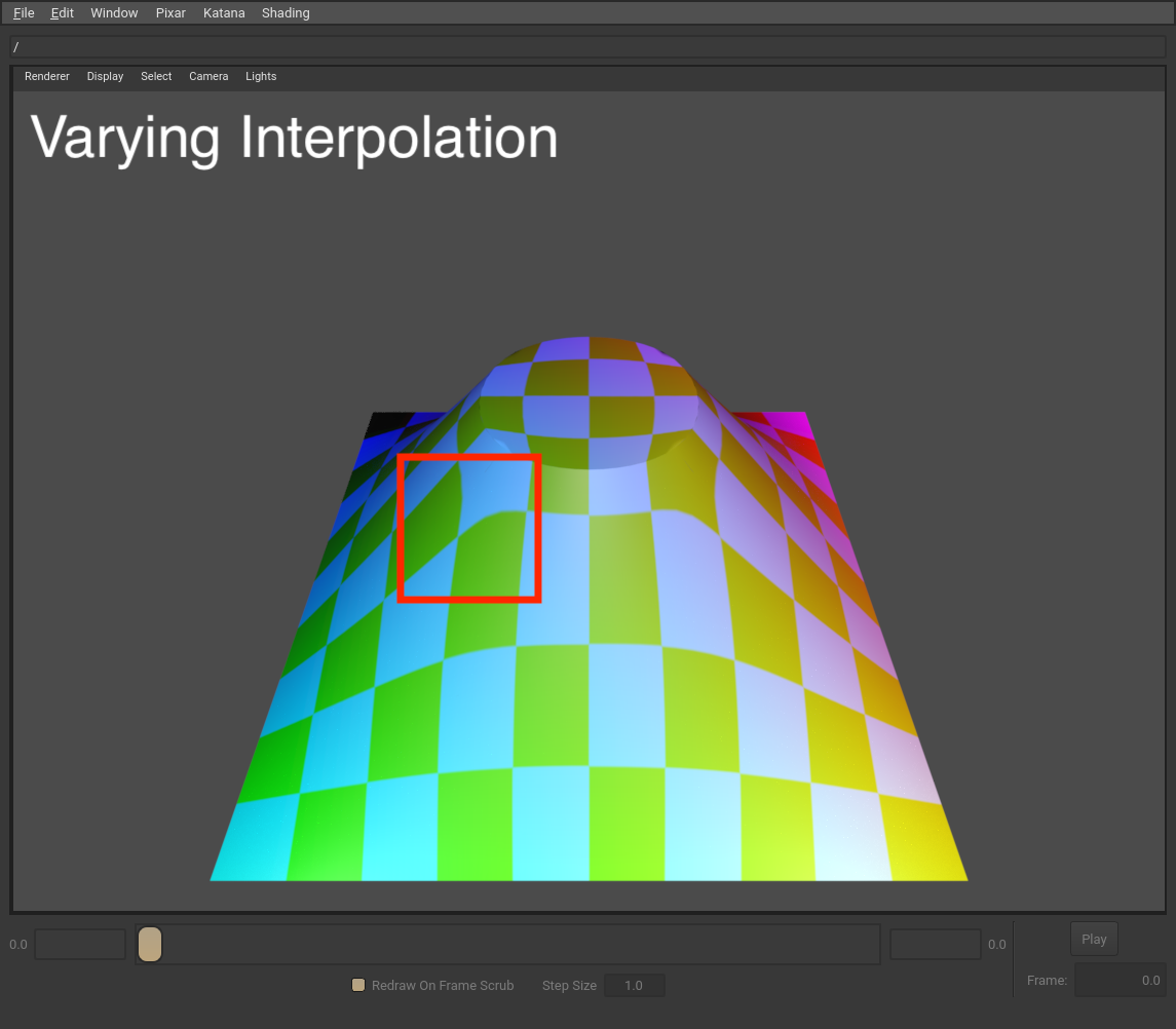
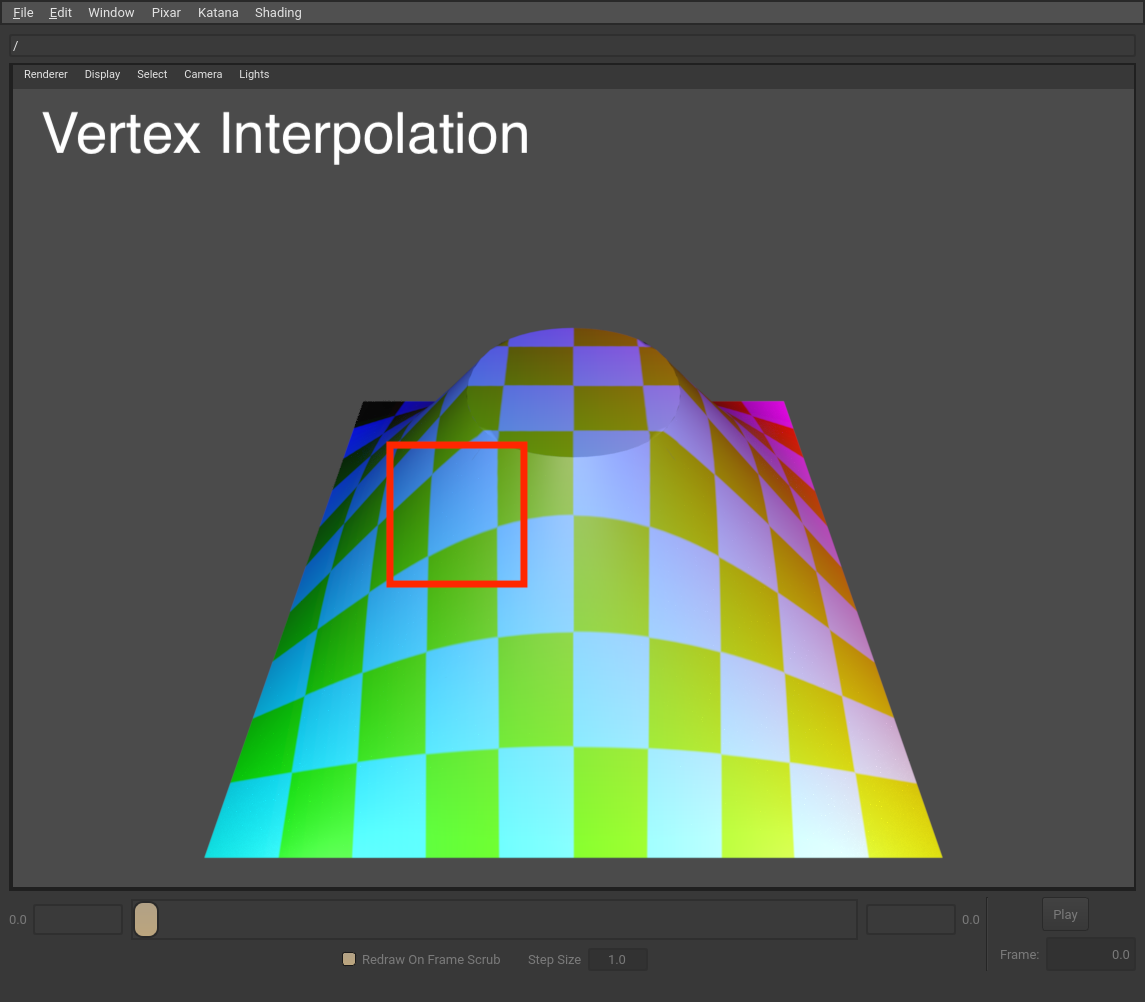
Here is another example showing the difference between varying and vertex interpolation using a more complex surface and a texture. Notice how the texture appears slightly more “stretched” along the edge of a patch in the highlighted area of the varying interpolation example.

Note

If you’re working with polygonal mesh data that is explicitly not intended to be subdivided, you should use varying interpolation in addition to setting the mesh subdivision scheme to none. This will ensure that the mesh renders identically whether a renderer supports subdivision or not.

faceVarying Interpolation

For polygons and subdivision surfaces, faceVarying interpolation allows you to specify different elements for each face-vertex. Bilinear interpolation (with additional rules for subdivision surfaces, see below) is used for interpolation between the elements. faceVarying interpolation allows you to specify different elements for each face-vertex of each point on the Mesh, which allows you to achieve unique interpolation of primvar elements across each face without affecting interpolation of primvar elements on surrounding faces. For example, you can use faceVarying interpolation to create discontinuous vertex UVs to create a “seam” in your texture-coordinate mapping, if you wanted to emulate wrapping a label around a cylinder. As another example, faceVarying interpolation is often used with indexed primvars to describe mesh topology discontinuities.

Note

Currently, faceVarying interpolation is not support for basis curves.

For Mesh prims, you’ll provide a primvar array with one element for each face-vertex of each face, with the order of the primvar array matching the order of the Mesh faceVertexIndices array.

In our example mesh with two faces, we author an array with eight colors (matching the Mesh faceVertexIndices array count and order). Hydra/Storm renders the Mesh with varying interpolation going from red to blue for each face.

#usda 1.0
(
)

def Mesh "faceVarying"
{
    float3[] extent = [(-1, 0, 0), (1, 1, 0)]
    point3f[] points = [(-1, 0, 0), (-1, 1, 0), (0, 1, 0), (0, 0, 0), (1, 1, 0), (1, 0, 0)]
    int[] faceVertexCounts = [4, 4]
    int[] faceVertexIndices = [3, 2, 1, 0, 5, 4, 2, 3]

    color3f[] primvars:displayColor = [(0,0,1), (0,0,0.75), (0.75,0,0), (1,0,0),
                                       (0,0,1), (0,0,0.75), (0.75,0,0), (1,0,0)] (
        interpolation = "faceVarying"
    )

    double3 xformOp:translate = (0, 0, -10)
    uniform token[] xformOpOrder = ["xformOp:translate"]
}

You can further control how elements are interpolated for subdivision surfaces through the faceVaryingLinearInterpolation Mesh attribute. See the Mesh API doc and OpenSubdiv documentation on FaceVarying Primvars for more details on the different rules. The previous example configured to use linear interpolation for the boundaries and interior of each face would look like the following.

#usda 1.0
(
)

def Mesh "faceVarying"
{
    float3[] extent = [(-1, 0, 0), (1, 1, 0)]
    point3f[] points = [(-1, 0, 0), (-1, 1, 0), (0, 1, 0), (0, 0, 0), (1, 1, 0), (1, 0, 0)]
    int[] faceVertexCounts = [4, 4]
    int[] faceVertexIndices = [3, 2, 1, 0, 5, 4, 2, 3]

    color3f[] primvars:displayColor = [(0,0,1), (0,0,0.75), (0.75,0,0), (1,0,0),
                                       (0,0,1), (0,0,0.75), (0.75,0,0), (1,0,0)] (
        interpolation = "faceVarying"
    )

    # Configure the face-varying interpolation rule for this surface
    token faceVaryingLinearInterpolation = "all"

    double3 xformOp:translate = (0, 0, -10)
    uniform token[] xformOpOrder = ["xformOp:translate"]
}

Primvars and the Scene Namespace

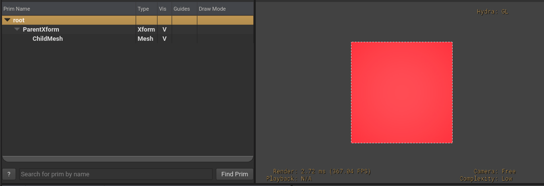
Primvars have a characteristic different from most USD attributes in that primvars will get “inherited” down the scene namespace. Regular USD attributes only apply to the prim on which they are specified, but primvars implicitly also apply to all child imageable prims (unless the child prims have their own opinions about those primvars). This allows for sparse authoring of sharable data in use-cases that require broadly authoring values for all Gprims in a complex model hierarchy.

Note that only constant interpolation modes are applied down the namespace. This restriction prevents unintentional and hard-to-diagnose asset breakage if topology-dependent interpolation modes are propagated down the namespace and the Mesh topology changes.

In the following example, ParentXform has an opinion for the displayColor primvar (using constant interpolation). ChildMesh has no opinion authored for the displayColor primvar, but will get rendered with the primvar value from its parent.

#usda 1.0
(
)

def Xform "ParentXform"
{
    color3f[] primvars:displayColor = [(1, 0, 0)] (
        interpolation = "constant"
    )

    double3 xformOp:translate = (0, 0, -10)
    uniform token[] xformOpOrder = ["xformOp:translate"]

    def Mesh "ChildMesh"
    {
        float3[] extent = [(0, 0, 0), (1, 1, 0)]
        point3f[] points = [(0, 0, 0), (0, 1, 0), (1, 1, 0), (1, 0, 0)]
        int[] faceVertexCounts = [4]
        int[] faceVertexIndices = [3, 2, 1, 0]

        # Primvar inherits down namespace, so this child prim automatically gets primvar

        double3 xformOp:translate = (0.5, -1, 0)
        uniform token[] xformOpOrder = ["xformOp:translate"]
    }
}

When using scene instancing, primvars are implicitly applied down the hierarchy for instances, as expected. You can author overriding values for primvars on the instance prim and these edits will be implicitly applied for that instance. Note that you cannot override primvars on child prims of instance prims, as properties on descendant prims beneath instance prims is not allowed by scene instancing.

Indexed Primvars

Primvars support indexed data, so data can be referred to by index rather than repeating the full elements, thereby reducing memory usage. A common use-case is using a primvar to describe surface normals for a Mesh, where several vertices use the same normal vector. In this scenario, it would be much more efficient to use primvar indices rather than duplicating the normals in the primvar array.

As an example, we can replicate the faceVarying interpolation example shown earlier, but use indices to avoid having to repeat duplicate colors:

#usda 1.0
(
)

def Mesh "faceVarying"
{
    float3[] extent = [(-1, 0, 0), (1, 1, 0)]
    point3f[] points = [(-1, 0, 0), (-1, 1, 0), (0, 1, 0), (0, 0, 0), (1, 1, 0), (1, 0, 0)]
    int[] faceVertexCounts = [4, 4]
    int[] faceVertexIndices = [3, 2, 1, 0, 5, 4, 2, 3]

    color3f[] primvars:displayColor = [(0,0,1), (0,0,0.75), (0.75,0,0), (1,0,0)] (
        interpolation = "faceVarying"
    )
    # Use primvar indices to avoid duplicate elements in primvars array
    int[] primvars:displayColor:indices = [0,1,2,3,0,1,2,3]

    double3 xformOp:translate = (0, 0, -10)
    uniform token[] xformOpOrder = ["xformOp:translate"]
}

Note that indices refer to elements in the primvar, which in this example (and in most use-cases) equates to values in the primvar array. However, if the element size of the primvar is greater than 1, an index refers to an element made up of more than 1 primvar array value. See element size for an example.

Primvars using faceVarying interpolation can use indexing to unambiguously define discontinuities in their functions at edges and vertices, along with using faceVarying linear interpolation rules, as described in OpenSubdiv documentation on FaceVarying Primvars.

Indexed Primvars and Attribute Blocks

While primvars are accessible as attributes, you should avoid directly using attribute blocks on a primvar. This is because an attribute block on a primvar will only block the primvar elements, but not the primvar indices (which, as we saw above, are encoded in a separate attribute so that they can vary over time, when desired). Instead, use the BlockPrimvar() API from UsdGeom.PrimvarsAPI which blocks primvar elements and indices.

Using the faceVarying example with primvar indices from earlier, if we just blocked the primvar as an attribute:

stage = Usd.Stage.Open("faceVarying-example.usda")

prim = stage.GetPrimAtPath("/faceVarying")

primvar_api = UsdGeom.PrimvarsAPI(prim)

# If you call Block() on the primvar attribute, this will only block the
# elements, not the indices

primvar = primvar_api.GetPrimvar("primvars:displayColor")
primvar.GetAttr().Block()

print(stage.ExportToString())

The flattened stage will have primvars:displayColor set to None, but primvars:displayColor:indices still set to our authored array of indices:

def Mesh "faceVarying"
{
    float3[] extent = [(-1, 0, 0), (1, 1, 0)]
    int[] faceVertexCounts = [4, 4]
    int[] faceVertexIndices = [3, 2, 1, 0, 5, 4, 2, 3]
    point3f[] points = [(-1, 0, 0), (-1, 1, 0), (0, 1, 0), (0, 0, 0), (1, 1, 0), (1, 0, 0)]
    color3f[] primvars:displayColor = None (
        interpolation = "faceVarying"
    )
    int[] primvars:displayColor:indices = [0, 1, 2, 3, 0, 1, 2, 3]
    double3 xformOp:translate = (0, 0, -10)
    uniform token[] xformOpOrder = ["xformOp:translate"]
}

This could cause subtle problems if later the primvar elements are re-authored without knowing how the indices are set. If instead we call BlockPrimvar():

primvar_api.BlockPrimvar("primvars:displayColor")

The primvar elements and indices are both set to None.

def Mesh "faceVarying"
{
    float3[] extent = [(-1, 0, 0), (1, 1, 0)]
    int[] faceVertexCounts = [4, 4]
    int[] faceVertexIndices = [3, 2, 1, 0, 5, 4, 2, 3]
    point3f[] points = [(-1, 0, 0), (-1, 1, 0), (0, 1, 0), (0, 0, 0), (1, 1, 0), (1, 0, 0)]
    color3f[] primvars:displayColor = None (
        interpolation = "faceVarying"
    )
    int[] primvars:displayColor:indices = None
    double3 xformOp:translate = (0, 0, -10)
    uniform token[] xformOpOrder = ["xformOp:translate"]
}

Primvar Element Size

In the examples in this doc we use the term “elements” to mean single values in a primvar’s value array. However, primvars can optionally specify elementSize, which sets how many consecutive values in the primvar array should be treated as a single element to be interpolated over a Gprim. If not set, a primvar’s elementSize defaults to 1.

As a simple example, we have a prim with a primvar that has a value array of strings, and an elementSize of 2. The primvar is indexed, so we can inspect the flattened primvar to show how each indexed element refers to a pair of strings from the strings array.

#usda 1.0
(
)

def Cube "TestPrim"
{
    string[] primvars:testPrimvar = ["element1-partA", "element1-partB", "element2-partA", "element2-partB"] (
        elementSize = 2
    )
    int[] primvars:testPrimvar:indices = [0, 1, 0]
}

The flattened primvar will look like:

[element1-partA, element1-partB, element2-partA, element2-partB, element1-partA, element1-partB]

Notice how the primvar indices refer to pairs of values in the value array – the “1” index refers to the third and fourth items in the values array.

Generally, the default element size of 1 will work for most use-cases. However you may encounter use-cases where you need to communicate an aggregate element to a renderer (e.g. representing spherical harmonics using nine floating-point coefficients) using larger element sizes.